Ashwin's Blog

Tracking Rural Settlements Using Satellite Images

Building A Segmentation Model

The use of satellite imagery has had a direct impact on improving the standards of human life. Real-time weather monitoring, disaster management through efficient resource mobilization and measuring shifts in tectonic plates are technologies that often gets taken for granted by the average person but is only made possible by years of investment in satellites.

Satellite technology has come so far, that the said average person can get real-time satellite images by making a simple API call from a laptop. As developers, we can use these high quality satellite images to tackle some interesting problems.

The Problem Statement

There are several NGOs that work to improve the living conditions of humans, especially in third world countries. For these NGOs to complete their mission, they have to reach these rural settlements first, which are spread across several hundred kilometres. Currently, they rely on manual labor by scrolling through Google Maps and locating rural settlements. Is there a way to automate this using Machine Learning?

What Is Semantic Segmentation?

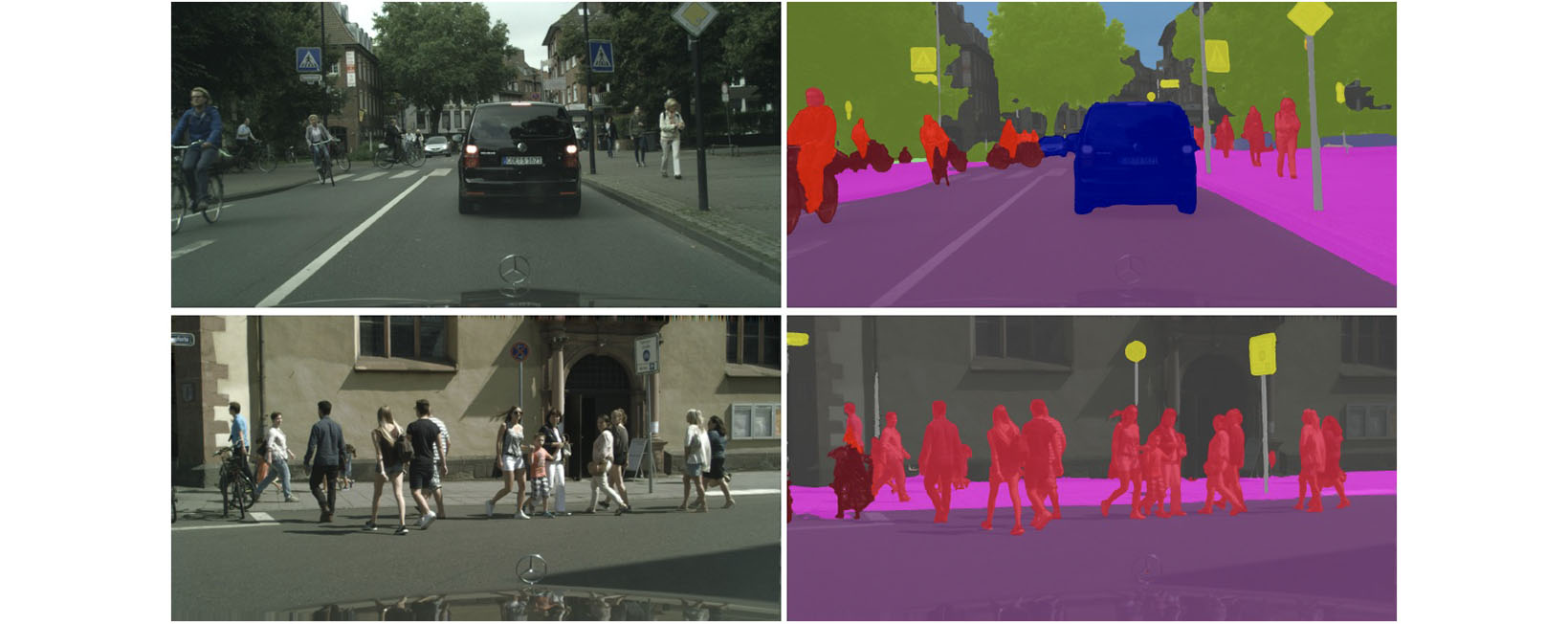
Input image and ground truth for semantic segmentation.

Semantic Segmentation is a problem statement within Computer Vision where we classify each and every pixel within the image. Unlike classification, we need dense pixel-wise predictions from our model. Above are two examples of input and output.

Increasing training data

We have very limited training data (which can be fetched as an API call from various open source web APIs, we will use data obtained from the Mapbox API) and thus need to use certain techniques as pre-processing steps before we plug the data in our model.

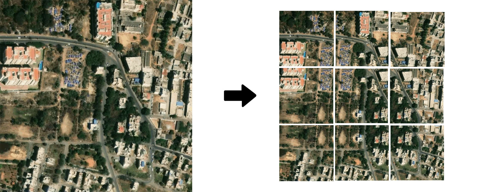
Sliding window technique to generate more training data

We need our input images to be 224 x 224 x 3 (We will go into details about in a bit) and the images we get from the Mapbox API call are of the dimension 600 x 600 x 3. We use the overlapping sliding window approach and split the image into 9 images of the required size. The image below tries to represent how this ‘splitting’ works.

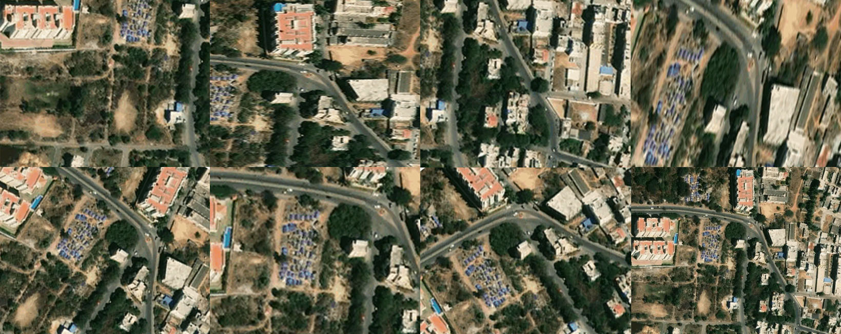
Data augmentation to generate more training data

To make the most out of our less training data, we will “augment” them via a number of random transformations, so that our model would never see the exact same picture more than once. We can apply a number of image transformations including random rotation and sheer operations. Keras allows us to instantiate generators of augmented image batches and their masks and lets us to plug it directly into our training model.

Using these methods, we end up with 90x the amount of data we originally had (9 sliding windows * 10 augmentations)

Segmentation Model

Silimar to what happened with image classification, deep learning had a lot of success on segmentation problems. In 2014, Long et al. introduced Fully Convolutional Network (FCN) which put forth Convolutional Neural Networks training end-to-end to make dense predictions by ditching the conventional fully connected layers. Although FCNs were a novel technique to train Convolutional Neural Networks, they produced very course looking output. One of the main problems with using CNNs for segmentation is the pooling layers which throw information, information which needs to be preserved to produced fine-grained segmentation masks. Since, there have been many efforts made to come up with better architectures.

One such popular architecture is the U-Net, a encoder-decoder network that first reduces spatial dimension in the encoder and recovers spatial information through the decoder with the help of maps of maxpooling indices. We use a U-Net because it has a lot of pre-trained models as it is the top choice for solving segmentation problems in the Kaggle community.

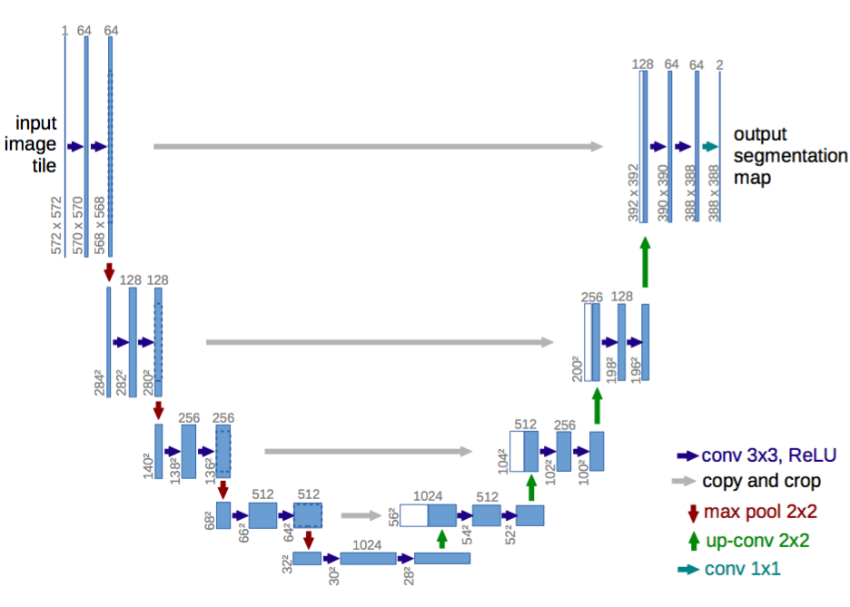
U-Net: An encoder-decoder architecture.

Here is the source code to build a U-Net model in Keras.

from keras.models import Model
from keras.layers import Input, merge, Convolution2D, MaxPooling2D, UpSampling2D
from keras.layers.normalization import BatchNormalization
from keras.layers.core import Dropout, Activation
from keras import backend as K

# Number of image channels (for example 3 in case of RGB, or 1 for grayscale images)
INPUT_CHANNELS = 3
# Number of output masks (1 in case you predict only one type of objects)
OUTPUT_MASK_CHANNELS = 1

def double_conv_layer(x, size, dropout, batch_norm):
    conv = Convolution2D(size, 3, 3, border_mode='same')(x)
    if batch_norm == True:
        conv = BatchNormalization(mode=0, axis=1)(conv)
    conv = Activation('relu')(conv)
    conv = Convolution2D(size, 3, 3, border_mode='same')(conv)
    if batch_norm == True:
        conv = BatchNormalization(mode=0, axis=1)(conv)
    conv = Activation('relu')(conv)
    if dropout > 0:
        conv = Dropout(dropout)(conv)
    return conv

def UNET_224(dropout_val=0.05, batch_norm=True):
    inputs = Input((INPUT_CHANNELS, 224, 224))
    conv1 = double_conv_layer(inputs, 32, dropout_val, batch_norm)
    pool1 = MaxPooling2D(pool_size=(2, 2))(conv1)

    conv2 = double_conv_layer(pool1, 64, dropout_val, batch_norm)
    pool2 = MaxPooling2D(pool_size=(2, 2))(conv2)

    conv3 = double_conv_layer(pool2, 128, dropout_val, batch_norm)
    pool3 = MaxPooling2D(pool_size=(2, 2))(conv3)

    conv4 = double_conv_layer(pool3, 256, dropout_val, batch_norm)
    pool4 = MaxPooling2D(pool_size=(2, 2))(conv4)

    conv5 = double_conv_layer(pool4, 512, dropout_val, batch_norm)
    pool5 = MaxPooling2D(pool_size=(2, 2))(conv5)

    conv6 = double_conv_layer(pool5, 1024, dropout_val, batch_norm)

    up6 = merge([UpSampling2D(size=(2, 2))(conv6), conv5], mode='concat', concat_axis=1)
    conv7 = double_conv_layer(up6, 512, dropout_val, batch_norm)

    up7 = merge([UpSampling2D(size=(2, 2))(conv7), conv4], mode='concat', concat_axis=1)
    conv8 = double_conv_layer(up7, 256, dropout_val, batch_norm)

    up8 = merge([UpSampling2D(size=(2, 2))(conv8), conv3], mode='concat', concat_axis=1)
    conv9 = double_conv_layer(up8, 128, dropout_val, batch_norm)

    up9 = merge([UpSampling2D(size=(2, 2))(conv9), conv2], mode='concat', concat_axis=1)
    conv10 = double_conv_layer(up9, 64, dropout_val, batch_norm)

    up10 = merge([UpSampling2D(size=(2, 2))(conv10), conv1], mode='concat', concat_axis=1)
    conv11 = double_conv_layer(up10, 32, 0, batch_norm)

    conv12 = Convolution2D(OUTPUT_MASK_CHANNELS, 1, 1)(conv11)
    conv12 = BatchNormalization(mode=0, axis=1)(conv12)
    conv12 = Activation('sigmoid')(conv12)

    model = Model(input=inputs, output=conv12)
    return model

Results

Here is a mask that is generated by the model and as we can see, this mask is a perfect fit in terms of segmenting out the rural community. The output of the model was fed into a CRF to get a more fine-grained mask.

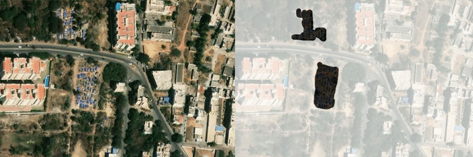
Left: Input Image, Right: Predicted Mask (overlayed on the image)

Conclusion

There are superior algorithms for semantic segmentation like Mask R-CNN. It is just easier to use a pre-trained netwrok and fine-tune the last layers, a method which is orders of magnitude cheaper when it comes to computational resources. U-Net is an excellent choice for segmentation problems since it has the support of the entire community of Kaggle. A more in-depth post about Semantic Segmentation will be coming soon. Stay tuned!